
You probably came across the cost variance (CV) when you had been reading about earned value management and variance analysis. Whether you are controlling the cost of your project or preparing for the PMP exam – being familiar with the CV is essential to master project cost management.
This article introduces the concept of cost variance. It also contains the definitions of the different CV types, their formulas as well as an example and a cost variance calculator.
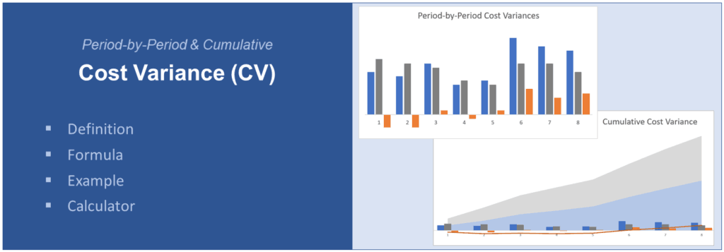
What Is Cost Variance?
Cost Variance (CV) is an indicator of the difference between earned value and actual costs in a project. It is a measure of the variance analysis technique which is a part of the earned value management methodology (EVM; source). Some argue that is an element of the earned value analysis (EVA) as well. However, this is not exactly accurate – EVA is rather the technique where the input data (i.e. the cost and value indicators) for the calculation of cost and schedule variances are determined.
There are three types of cost variances:
- point-in-time or period-by-period cost variance,
- cumulative cost variance, and
- variance at completion (VAC), as a specific type of the cumulative cost variance.
The following sections shed a light on their definitions and differences of these types.
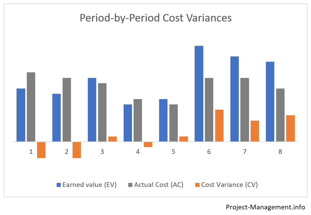
What Is Point-in-time / Period-by-Period Cost Variance?
This is the simplest type of cost variance: It basically refers to the difference between actual cost and earned value within one period. Thereby, it does not take any indicators or variances of previous or future variances into account.
For instance, if you are in month 4 of a project, you would calculate the point-in-time cost variance of that period by using the actual cost (AC) and earned value (EV) of the 4th month only.
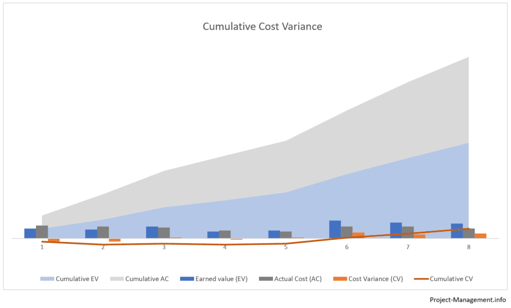
What Is Cumulative Cost Variance?
The cumulative CV is a measure for the cumulative difference of the cumulative earned value and actual cost figures of several, usually consecutive, periods.
If a project manager intends to calculate the cumulative cost variance of the 4th month of a project, for instance, she/he will have to calculate the cumulative earned value (EV) and the cumulative actual cost (AC) of the 4th and the previous months first.
In other words, the cumulative cost variance of the 1st to the 4th month is the difference between the sum of EV(1)+ EV(2)+EV(3)+EV(4) and the sum of AC(1)+AC(2)+AC(3)+AC(4).
What Is Variance at Completion (VAC)?
The variance at completion is the cumulative cost variance at the end of the project. The calculation parameters are the budget at completion (BAC) and the actual or estimated cost at completion (EAC). The VAC is often used as a measure of the forecasting techniques – you will find more details in this article on the estimate at completion (EAC).
How Is Cost Variance Calculated?
The basic formula for calculating the cost variance is:
CV = EV – AC,
where:
EV = Earned value;
AC = Actual cost.
Earned value (EV) refers to the part of the budget allocated to the part of the work that has been completed in a period or cumulatively over several periods.
The actual cost (AC) is the amount of cost or resources that has been incurred to perform the authorized work. It can relate to a single or several periods (cumulative AC)
This formula needs to be adapted for the different types of cost variances. While the basic calculation – the difference of EV and AC – is basically the same, the input parameters are replaced as follows.
How Is the Period-by-Period Cost Variance Calculated?
The period-by-period or point-in-time cost variance is calculated by using the basic formula with input parameters that refer to a single period:
CV(period) = EV(period) – AC(period)
The input parameters – EV and AC – relate to the work performed and the cost incurred in the reference period. They do not consider the numbers for any other period.
How Is the Cumulative Cost Variance Calculated?
The cumulative cost variance uses the basic formula with cumulative input parameters over several periods:
CV(cumulative) = EV(cumulative) – AC(cumulative)
or CV(cumulative) = Sum of CV(all
periods),
where: CV(all periods) represents all point-in-time CVs of the periods in scope.
The cumulative cost variance is often calculated for a time horizon from the beginning of a project to the most recent period. However, it can also refer to any other combination of periods, e.g. a cumulative cost variance could be calculated for the months 2 to 4 which would not take the first month nor any period after the 4th month into account.
What Is the Meaning of the Calculated Cost Variance Values?
The value of a calculated cost variance falls into one of the following 3 value ranges. Each of them has a different meaning:
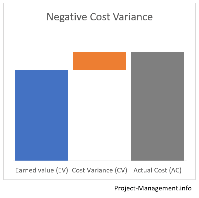
- a negative cost variance (CV < 0) indicates a cost overrun,
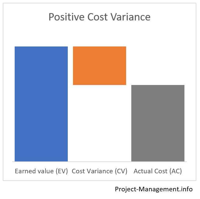
- a positive cost variance (CV > 0) indicates that the earned value exceeds the actual cost, and
- a cost variance of 0 which means that the budget is met, i.e. the actual cost is equivalent to the earned value.
Calculator for Cost Variances (Period-by-Period or Cumulative CV)
Use this calculator if you wish to calculate the period-by-period or cumulative cost variance of your project.
If you need to determine the cumulative cost variance, fill in the cumulative earned value and cumulative actual cost (make sure that both values relate to the same scope of periods). For a single period, populate AC and EV with the values for that particular period.
Examples of a Cost Variance Calculation and Analysis
The following 2 examples illustrate the calculation and the use of cost variances in a project. As these variances are often used together with the cost-performance index (CPI) – you will find more details in the corresponding example in this CPI article. Note that the input numbers in the CPI article are consistent with these examples.
Example 1: A Simple Calculation of Cumulative and Point in Time Cost Variances
In the first example, the PMO’s earned value analysis produced the following numbers:
| Month 1 | Month 2 | Cumulative numbers (month 2) | |
| Planned Value | 50 | 150 | 200 |
| Earned Value | 60 | 130 | 190 |
| Actual Cost | 50 | 170 | 220 |
Calculation of Cost Variances
The project manager calculates 2 cost variance types: the cumulative and the point-in-time cost variances, using the formula AC = EV – AC.
| Month 1 | Month 2 | Cumulative numbers (month 2) | |
| Earned Value | 60 | 130 | 190 |
| Actual Cost | 50 | 170 | 220 |
| Cost Variance (CV) per period | 60 – 50 = 10 | -130 – 170 = -40 | – |
| Cost Variance, cumulative | – | – | 190 – 220 = -30 [or: 10 + (-40) = -30] |
Interpretation of the Calculated CV
The cumulative cost variance is negative. This means that the total costs that have been incurred so far exceed the earned value by 30.
This difference between earned value and actual cost in this example is actually not insignificant. Calculating the cost-performance index and determining the to-complete performance index can help analyze this result and assess its impact on the overall project.
Looking at the period-by-period cost variances leads to a more differentiated picture. While the first month’s cost variance was positive (i.e. the earned value exceeded the actual cost), it turned eventually negative in the 2nd month.
In this case, the calculation of point-in-time cost variances per period – in addition to the cumulative cost variance – can give the project manager a hint where to look for the root causes of the cost overrun.
Example 2: Case Study of a Project in a Turnaround Situation
In the second example, the PMO has determined the following numbers for the first 3 months of a project:
| Month 1 | Month 2 | Month 3 | Cumulative | |
| Planned Value | 100 | 130 | 200 | 430 |
| Earned Value | 60 | 120 | 220 | 400 |
| Actual Cost | 90 | 150 | 200 | 440 |
Calculating the Cumulative and Period-by-Period CV
The project manager is calculating the cost variances as follows:
cumulative CV = 400 – 440 = -40
Again, the negative cumulative cost variance indicates a cost overrun after the first 3 months of the project.
However, breaking it down into a period-by-period analysis leads to the following figures:
| Month 1 | Month 2 | Month 3 | Cumulative | |
| Cost Variance per period | -30 | -30 | 20 | -40 |
Interpretation of the Cost Variances
The cost variances changed from CV (m1) = -30 in the first month to a positive CV (m3) = +20 in the third month.
Such cost developments are not unusual given that projects and teams may require some ‘settling in’ time before they can leverage their full performance potential. Without prejudice to other internal and environmental aspects, the change to a positive point-in-time cost variance in the 3rd month could be an indicator of a positive turn-around of the project’s performance.
The project manager might want to further assess and facilitate the sustainability of this positive development.
Conclusion
The cost variance is one of the fundamental measures of the variance analysis which is part of the earned value management method introduced in PMI’s Project Management Body of Knowledge (source: PMBOK®, 6th ed., ch. 7.4.2.2 Data Analysis, p. 261-264).
The CV itself indicates whether the cost incurred for work performed in one or more periods of a project meets, exceeds or falls below the budgeted amount.
While this measure relates to the cost of a project, the corresponding indicator for the project schedule is the schedule variance (SV). Variations of these measures are the schedule performance index and the cost performance index – you will find more details on these indexes in this article.