
When you are in the process of controlling the schedule of your project, or when you are preparing for your PMP exam, you will likely make use of the Schedule Variance (SV) at some point. This is one of the key indicators of the variance analysis which is part of the earned value management of a project.
In this article, we are sharing the definition, formula and types of schedule variance, supplemented with a comprehensive example and a free SV calculation tool.
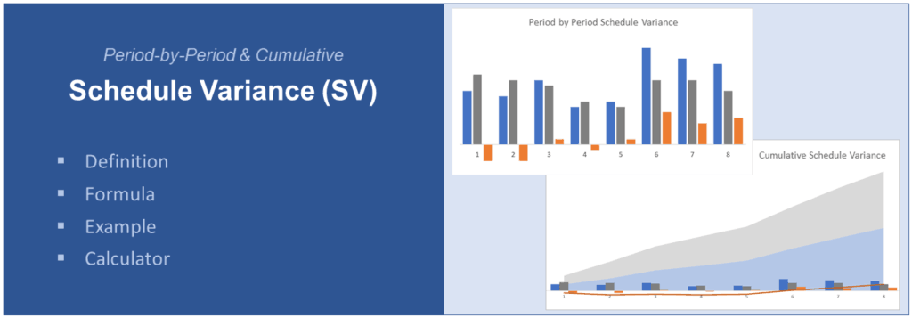
- What Is Schedule Variance?
- How Is Schedule Variance Calculated?
- What Is the Meaning of the Calculated Schedule Variance Values?
- Calculator for Schedule Variances (Period-by-Period or Cumulative SV)
- Examples of Schedule Variance Calculation and Analysis
- Conclusion
What Is Schedule Variance?
Schedule Variance (SV) is a term for the difference between the earned value (EV) and the planned value (PV) of a project. It is used a measure of the variance analysis that forms an element the earned value management techniques. An alternative but less common classification of this technique is earned schedule management or analysis.
The schedule variance indicates whether the performance – i.e. the authorized work performed – exceeds, falls below or is equal to the planned performance. Projects that apply the PMI methodology use SV typically in their “control schedule” process.
There are two different types of schedule variances:
- point-in-time or period-by-period schedule variance and
- cumulative schedule variance.
While both types share the same calculation approach, their meanings can differ significantly. Learn more about these differences in the following sections and the examples below.
The corresponding indicator for the cost controlling in a project is called cost variance.
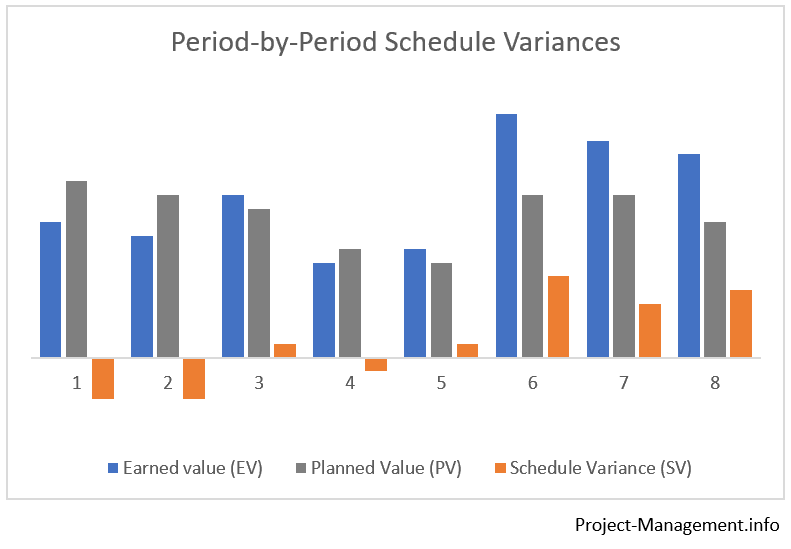
What Is Point-in-time / Period-by-Period Schedule Variance?
Point-in-time or period-by-period schedule variance refers to the difference between earned value (as observed and measured in a period) and planned value with respect to a single period. Variances of other periods, such as excesses or shortfalls, are not considered.
Example: If you are calculating the schedule variance for the 2nd month, for instance, you would not take the SV of the 1st and 3rd month into account.
This is the key difference to the cumulative schedule variance. Read on for more details.
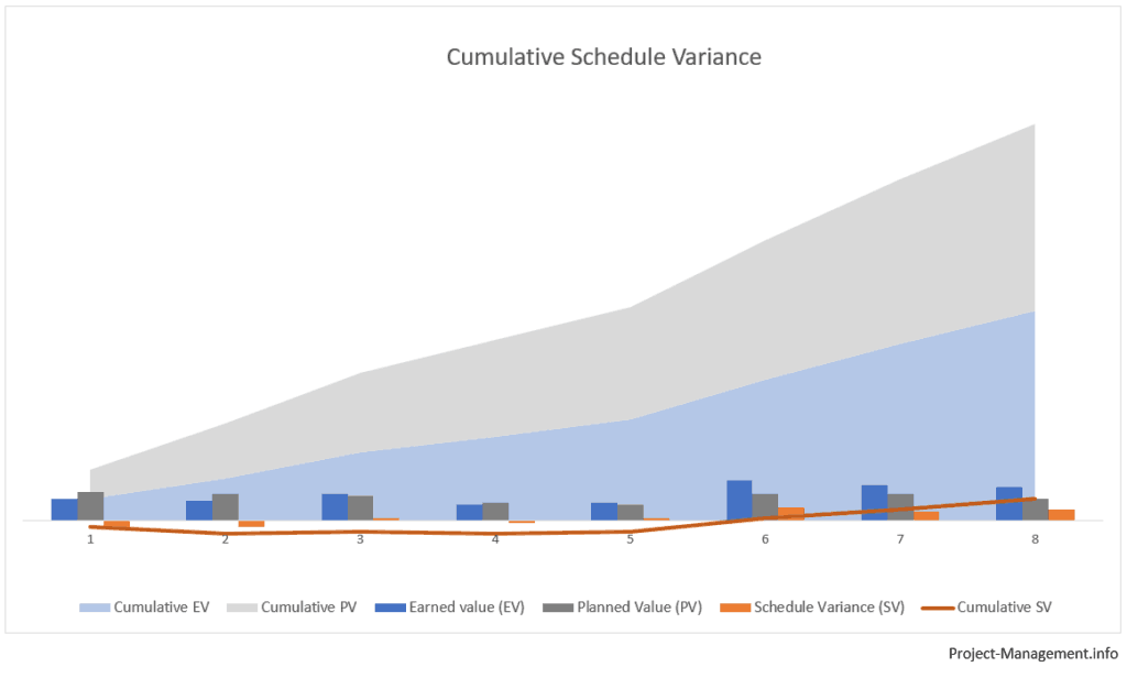
What Is Cumulative Schedule Variance?
The cumulative SV refers to the difference between earned and planned value over several – mostly consecutive – periods. It is either the sum of the point-in-time schedule variances of all periods in scope or the difference of the sum of EVs and the sum of PVs for these periods.
Example: If you intend to calculate the cumulative schedule variance for the periods 1 to 3, for instance, you will sum up the period-by-period SVs of the periods 1, 2 and 3. Alternatively, you can determine the sum of EV(per.1) + EV(per.2) + EV(per.3) and deduct the sum of PV(per.1) + PV(per.2) + PV(per.3) which results in the cumulative schedule variance.
How Is Schedule Variance Calculated?
You can use the following formula to calculate the schedule variance (SV) of one or several periods:
SV = EV – PV,
where:
EV = Earned value;
PV = Planned value.
Earned value is determined in the earned value analysis. It indicates how much of the authorized work (measured in allocated budget) has been completed within a single or a time frame of several periods.
Planned value is the part of the budget that is allocated to the amount of work that should have been completed in a period or several periods. It is derived from the project baseline (or project plan).
Both parameters must be denominated in the same unit – typically a currency unit (like $) or man-days – and refer to the same period(s).
You have probably noted that both the EV and the PV definitions imply two options: they can either refer to a single period or multiple periods. While the basic calculation is basically identical for either case, the basis of the parameters would be different. This is further explained in the following sections.
How Is the Period-by-Period Schedule Variance Calculated?
The calculation of the period-by-period or point-in-time schedule variance follows the previously introduced basic formula:
SV(period) = EV(period) – PV(period).
Earned value (EV) and planned value (PV) refer to a single period in this case.
How Is the Cumulative Schedule Variance Calculated?
For the cumulative schedule variance, the basic formula is used with input values for multiple periods:
SV(cumulative) = EV(cumulative) – PV(cumulative)
or SV(cumulative) = Sum of SV(all periods),
where SV(all periods) refers to all point-in-time SVs of the periods in scope.
It is common in projects that the cumulative schedule variance is measured for the first to the most recent period. However, it can also be calculated for a different time frame, e.g. the 2nd to 5th period of a project, if this information is required.
What Is the Meaning of the Calculated Schedule Variance Values?
Similar to other variance indicators in project management, the schedule variance comes with three potential value ranges that have their own respective meaning:
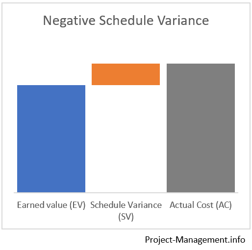
- A negative schedule variance (SV < 0) indicates that the project is behind the schedule, as earned value does not meet the planned value.
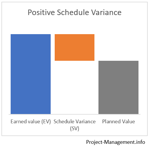
- A positive schedule variance (SV > 0) indicates that the earned value exceeds the planned value in the reference period(s), i.e. the project is ahead of the schedule.
- If the schedule variance is 0 this indicates that that the schedule baseline is met, i.e. the earned value is equal to the planned value.
Note that the values of the different types of SV may vary within the same project, depending on the reference period(s) that you have selected.
For instance, the SV of a single period can be negative while the cumulative schedule variance can as well be 0 or positive at the same time.
Calculator for Schedule Variances (Period-by-Period or Cumulative SV)
You can use this calculator to determine the schedule variance of your project. The values can either refer to a single period or cumulative, depending on the type of input parameters (EV and PV) that you provide.
Examples of Schedule Variance Calculation and Analysis
In the following 2 examples, we will guide you through the use and calculation of the schedule variance in certain project situations. You will find a corresponding example with identical EV and PV amounts in our article on the schedule performance index.
Example 1: A Simple Calculation of Cumulative and Point in Time Schedule Variances
In this example, the PMO has observed the following numbers as part of their ongoing earned value analysis.
| Month 1 | Month 2 | Cumulative (Month 2) | |
| Planned Value (PV) | 50 | 150 | 200 |
| Earned Value (EV) | 60 | 130 | 190 |
Calculation of Schedule Variances
To determine the variance, the planned value is subtracted from the earned value for each period. The same approach is applied to the cumulative numbers. The calculation and results are illustrated in this table.
| Month 1 | Month 2 | Cumulative (Month 2) | |
| Planned Value (PV) | 50 | 150 | 200 |
| Earned Value (EV) | 60 | 130 | 190 |
| Schedule Variance (SV) per period | 60 – 50 = 10 | 130 – 150 = -20 | |
| Schedule Variance, cumulative | 190 – 200 = -10 or: 10 + (-20) = 10 |
Interpretation of the Calculated SV
The project is slightly behind schedule which is indicated by the negative cumulative schedule variance of -10.
Considering the period-by-period numbers, a positive schedule variance is observed in the first period (earned value exceeds the planned value). However, the project missed its schedule baseline in month 2 where the planned value has not been met at all.
In practice, such a breakdown can be a good starting point for a further root cause analysis if the project fails to meet the schedule baseline.
Example 2: Case Study of a Project in a Turnaround Situation
This example illustrates how the numbers for a turnaround situation can look like. The following table shows the numbers for months 1 to 3 of a project.
| Month 1 | Month 2 | Month 3 | Cumulative (Month 3) | |
| Planned Value (PV) | 100 | 130 | 200 | 430 |
| Earned Value (EV) | 60 | 120 | 220 | 400 |
Calculating the Cumulative and Period-by-Period SV
For the cumulative schedule variance, the numbers of the last column are used and inserted into the previously introduced formula:
cumulative SV = 400 – 430 = -30
This negative cumulative SV indicates that the project is behind schedule after 3 months.
On a period-by-period basis, the schedule variance is as follows:
| Month 1 | Month 2 | Month 3 | Cumulative (Month 3) | |
| Schedule Variance (SV) | -40 | -10 | 20 | -30 |
Interpretation of the Schedule Variances
The schedule variances starter with a negative SV of -40 in the first month which was then managed down to -10 in month 2. The situation improved eventually with a positive SV of +20 in the third month.
While the project still fails to meet the overall schedule baseline, the breakdown by months shows a positive trend: the initially negative schedule variance improved incrementally over time.
If this development is sustainable and positive, or at least 0, variances can be retained, the project will have a realistic chance to be back on track within a few months. In practice this may also depend on other factors though.
Conclusion
The schedule variance is a key success measure in both the variance analysis as well as in the earned value management methodology as defined in PMI’s Project Management Body of Knowledge (source: PMBOK®, 6th edition, ch. 7.4.2.2 Data Analysis, p. 261-264).
In day-to-day project management, it is also relevant for project managers’ status reporting and communication with stakeholders.
As the schedule variance provides the absolute difference between the work performed and the scheduled work, it does not set this result in relation to the overall size of the project. This can be achieved by calculating the schedule performance index (SPI).
In case of negative variances, the to-complete-performance index (TCPI) can help quantify corrective measures that would be necessary to complete the project in time and budget. Read more about the TCPI in this article that also contains an illustrative example.