
When you perform a cost-benefit analysis and need to compare different investment alternatives with each other, you might consider using the net present value (NPV) as one of the profitability indicators. In project management, the NPV is commonly used and also listed in PMI’s Project Management Body of Knowledge (source: PMBOK®, 6th edition, part 1, ch. 1.2.6.4, p. 34). While the basic calculation – the sum of discounted cash flows – is comparatively easy, it is key to understand the assumptions, strengths and weaknesses of the NPV to make a reflected investment decision.
This article will introduce the net present value, its formula as well as the required assumptions. This includes the different components and pros and cons of this indicator and is further illustrated with 2 comprehensive examples. Thus, you will be able to apply the NPV in a sensible way when you compare different investment and project alternatives and when you present them to your stakeholders.
- What Is the Net Present Value? The Definition.
- The Net Present Value (NPV) Formula
- Components and Assumptions of the NPV Computation
- How to Calculate the Net Present Value in 6 Comprehensive and Understandable Steps
- Examples of NPV Calculations in Practice
- Advantages and Disadvantages of the NPV
- Conclusion
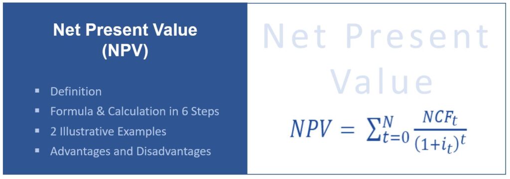
What Is the Net Present Value? The Definition.
The NPV represents the monetary value of a series of future cash flows by today. All future cash flows are therefore discounted with a predefined interest rate or discount rate. The NPV is part of the set of Discounting Cash Flows (DCF) methods.
The net present value is often used in the context of a cost-benefit analysis where it is a common indicator for the profitability of project or investment alternatives:
- A positive NPV suggests that the investment is profitable, i.e. the return exceeds the predefined discount rate).
- The NPV is negative if expenses are higher or occur earlier than the returns. Thus, the investment does not yield the
- A net present value of 0 indicates that the investment earns a return that equals the discount rate.
The Net Present Value (NPV) Formula
The formula for the calculation of the net present value is
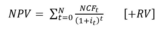
where:
NPV = Net Present Value
NCF = Net Cash Flow of a period
i = Discount Rate or Interest Rate
RV = Residual Value
N = Total Number of Periods
t = Period in which the Cash Flows occur
These parameters are determined by certain estimates and assumptions which are discussed in the following section.
Components and Assumptions of the NPV Computation
The formula consists of three different fundamental elements:
- the assumed cash flow of a period (for each period),
- the preset discount rate or interest rate (for each period),
- the residual value at the end of the projection (optional).
The NPV calculation takes the point in time into account at which cash flows occur. With a positive discount rate (which is by far the most common use), earlier cash flows impact the NPV more than those of later periods. This can lead to a negative NPV even if the simple non-discounted sum of cash flows is positive or 0.
Cash Flows
Cash Flows used for NPV computations are usually stemming from a business projection for an investment or a project opportunity. If you assess the value of a contract or a financial instrument with agreed upon payments, you will probably use those amounts though.
For instance, if you are planning a project with a one-year implementation time and 5 years use of the created result, your projected cash flows will be the estimated project cost in period 0 and 1 (initial investment) and the expected benefits and running cost as of period 1. Note that the scheduling of activities and, subsequently, cash flows will have an impact on the overall NPV (source).
For the calculation of the NPV, a net cash flow estimation is basically sufficient. It does not change the result whether you discount net cash flows or whether you discount gross inflows and outflows and offset the present values of both series.
However, if you intend to calculate the benefit-cost ratio in addition to the NPV, you will want to maintain a granular estimate of gross in- and outflows in your projection.
Discount Rate / Interest Rate
In the basic version of the NPV computation – which is usually applied for rough projections in early stages of a project – the discount rate remains constant for all periods and for all kinds of cash flows. It often represents the organization’s target return on investments or weighted average cost of capital (WACC).
In some areas, such as financial markets, the discount rates may vary among the different periods. They can, for instance, represent a market interest rate curve or swap rate curve. Those rates will then be used to price instruments and transactions.
In some cases, it may also be sensible to use different discount rates for different types of cash flows, e.g. distinguished into risk-free in- and outflows and those subject to higher risk.
An example of a very accurate yet rather complex approach is the project option valuation with net present value and decision tree analysis (read more on ScienceDirect).
While there are good reasons to do this in certain cases, complex calculation may often be over-engineered for small and mid-size projects, in particular in early stages. For such projects, interest rate changes or splits are often deemed less material compared to other assumptions and insecurities of a forecast.
Residual value
When you are projecting cash flows for a long time horizon, you will likely reach a point on the timeline where it is not reasonable to continue the detailed benefit and cost forecasting, e.g. when estimates lack accuracy or would require huge efforts. This is where the residual value becomes relevant (source).
The residual value represents the remaining value of an asset, a project result or an intangible good at the end of the time horizon of a projection.
In a construction project, for instance, a project controller might decide to determine detailed cash flows (or benefits and costs) for the years 1 to 10 of a projection. Subsequently, he would add a residual value to the projection in order to account for cash flows occurring in the years 11 and later or for the expected market value of the asset at the end of year 10.
There are 3 different types of residual values that are typically used:
- Discounted infinite series of cash flows / perpetuity,
- Expected market value (salvage value),
- Cost of disposal,
- Zero.
Infinite Series of Cash Flows / Perpetuity
This method is sensible for investments and assets that provide returns for an infinite time. Examples are certain types of assets with an infinite lifecycle, e.g. some financial instruments, (historic) buildings (arguable, but there are indeed historic buildings that lasted for centuries) or farmland. Their returns are reflected in a residual value that equals the present value of the perpetuity discounted to the last year of the forecast’s time horizon. It is calculated as follows:
Residual Value = Net Present Value = perpetuity / interest rate
The calculation of this value requires 2 assumptions: the constant perpetuity and the interest rate. The perpetuity reflects the constant net cash flow that is expected to occur after the detailed forecasting period.
The interest rate can be the discount rate of the NPV calculation, sometimes increased by an add-on to take the insecurity of long-term planning into account. If cash flows are expected to increase over time, e.g. in case of real estate investments, that growth rate is subtracted from the discount rate used for this calculation.
Most types of assets have a limited lifecycle though. The other approaches to determine their residual value are therefore more accurate. However, the present value of a perpetuity is sometimes also used for those types of investment as a proxy, usually involving a high interest rate (i.e. a lower present value) to account for the inaccuracy of the calculation.
Expected Market Value / Salvage Value as Residual Value
If it is intended to sell an asset at a future point in time, it is reasonable to include the forecasted market value in the NPV calculation. The future market value or salvage value needs to be estimated for this purpose.
Possible techniques include but are not limited to the extrapolation of past market value developments, the use of certain depreciation rules/curves or the expected future book value.
In project management, this residual value type is used, for instance, if a projection covers the entire lifetime of a product. A market value can be reasonable in cases where a project result is subject to a license requirement that allows for a usage shorter than the lifecycle of the assets purchased or created.
Project Residual Value of 0
A residual value of 0 is typically assumed if the projection horizon ends at the end of – or even beyond – the expected lifecycle of an asset or product. This may be applicable to fast-changing types of assets, e.g. software and electronic devices.
A residual value of 0 can also be a reasonable or conservative assumption if the future values or cash flows are highly uncertain or subject to a high degree of ambiguity.
Negative Residual Value due to Disposal Cost
Some types of assets will cause disposal costs when they are used up. These cost are also part of the cost-benefit assessment of such investments. Examples could be projects and investments that involve toxic material or constructions and structures that need to be removed eventually.
However, it is arguable whether these costs are classified as a negative residual value or a negative cash flow/cost in the detailed forecast. As either understanding leads mathematically to the same result, we will skip further elaboration on that discussion. One way or the other, it is just important not to forget the disposal cost when projecting cash flows.
How to Calculate the Net Present Value in 6 Comprehensive and Understandable Steps
Follow these 6 steps, use a calculation tool (such as Excel or our NPV calculator) and set aside a few hours to determine the NPVs of your project or investment options.
1. Determine the Expected Benefits and Cost of an Investment or a Project over Time
The basis for the calculation of the net present value are the projected benefits and cost over time. Depending on the characteristics of an investment or project option, you will likely want to involve subject matter experts who help you project the monetary value of the expected benefits and cost.
For this estimation, you can either develop your own estimation approach or refer to the following components that are commonly addressed in a forecast:
- Initial investment: Outflows, project cost, allocated staff and all other types of resources that are used to create the results or assets subject to this analysis. Depending on the time of their occurrence, these outflows can be allocated to or split into period 0 and period 1 of the projection.
- Recurring benefits / inflows from the investment or asset upon its completion.
- Recurring or running costs that are necessary to maintain the asset.
- One-off cost and one-off benefits / inflows within the time horizon.
All these components need to be estimated and allocated to periods (typically years). Once you have completed this granular forecast, proceed with the next step.
2. Calculate the Net Cash Flows per Period
Calculate the sum of all inflows and outflows for each period to determine the net cash flow of each period.
Alternatively, you can discount all gross cash flows (inflows as well as outflows) separately. Both ways will result in the same NPV.
3. Set and Agree the Discount Rate
Following our previous explanations, you will have to define an interest or discount rate which you will use for discounting the cash flows.
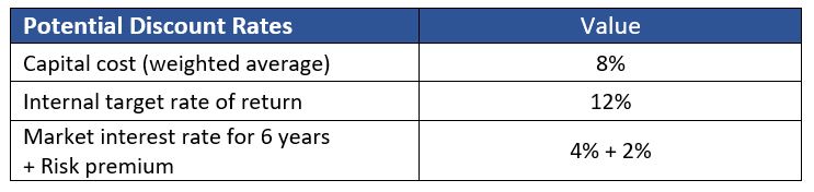
There are numerous options of how to come up with an appropriate discount rate. Some of the most common ways are:
- a company’s target return-on-investment rate;
- the cost of capital, i.e. the average rate a company needs to pay on its liabilities and as return on equity;
- a market rate, i.e. an interest rate financial instruments with similar tenor and riskiness would yield;
- a risk-adjusted rate, i.e. consisting of a base rate (such as risk-free interest rate or a company’s cost of capital) plus an add-on to take the specific risk of the endeavor into account.
In addition, interest rates can vary among the cash flow sources and periods: a swap or yield curve can be used to achieve an accuracy comparable to the valuation of financial markets instruments. If certain elements of the projected cash flows are more certain (e.g. cost) than other assumptions (e.g. sales revenue), the reflection of the different level of risk in the respective discount rate can be considered (in that case, step 2 needs to be modified in order to aggregate cash flows per period based on their riskiness).
In theory, there are many different options and assumptions involved in the determination of the interest rate. In practice though, a fixed interest rate – usually a company’s target return-on-investment rate – is the most common discount rate type for NPV calculations used to compare different project and investment options.
4. Determine the Residual Value
If necessary, estimate a residual value, as explained in the previous section. Consider the characteristics of the asset as well as the accuracy and reliability of a long-term forecast when you come up with a fitting residual value type. The following values can typically be used as residual values:
- a discounted infinite series of cash flows / perpetuity after the time horizon of the detailed projection,
- the expected market value (or salvage value) of an asset,
- the cost of disposal, or
- zero.
If you are choosing the present value of a perpetuity as your residual value, you will need to repeat step 3, the determination of a discount rate, for this calculation as well (read the details in the previous section).
In any case, make sure that the use and assumptions of a residual value are transparent and understandable for stakeholders. This is particularly recommended in cases where the residual value is one of the main drivers and components of the net present value. Thus, its rather rough assumptions might significantly impact investment decisions or the selection of project options.
5. Discount the Cash Flows of Each and Every Period
Discount the net cash flows of each period, following the abovementioned formula. Use the interest rate determined in step 3 and discount the residual value that you have calculated in the previous step.
Alternatively, you can discount gross cash flows first, e.g. separately for inflows and outflows or for different levels of riskiness.

6. Calculate the NPV as a Sum of Discounted Cash Flows
Whichever discounting method you have used in the previous step, the Net Present Value is always the sum of all your discounted cash flows.
You can then rank the different alternatives by profitability, starting with the highest NPV.
When you are using this result for your stakeholder communication, make sure that you do not only present the calculated figure but also its underlying assumptions. This will allow them to get a full picture of the projection and ensure the comparability of different investment or project options.
Examples of NPV Calculations in Practice
This section contains 2 examples, aiming to illustrate the application of NPV calculations to real-life situations. The first example comprises the comparison and selection of different project options. The second example elaborates on the use of perpetuities for infinite series of cash flows.
Example 1: Comparing Net Present Values of Different Software Solutions
The following example will help you understand the calculation and the parameters that affect the NPV.
Estimated Cash Flows and Agreed Discount Rate
During the pre-project phase, a project manager is asked to compare the financial effects of 3 alternative software solutions to facilitate the project sponsors’ decision-making.
The company’s expected return rate is 12% which is therefore the discount rate parameter of this NPV calculation. The investment and cost relate mainly to license, implementation, customizing and maintenance cost. The company intends to benefit from materialized efficiency gains as well as increased revenues as soon as the software helps enhance customer service.
The project manager is assessing the following 3 options for a new software solution:
- Option 1 comprises buying an off-the-shelf solution that requires some customizing and an implementation time of 1-2 years.
- Option 2 is more comprehensive software solution that needs a shorter implementation time yet requires a higher initial investment. It would be ready to produce positive cash flows as of year 1.
- Option 3 involves an in-house development project at a lower cost which however takes more time. Benefits are expected from year 2 on.
For all 3 cases, the software is expected to be replaced at the beginning of year 7 (i.e. immediately after year 6, the end of this projection) with no residual value.
Overview of Estimated Cash Flows
The subject matter experts involved in the cost-benefit analysis came up with the following estimated figures.
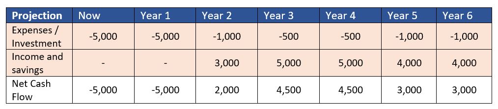
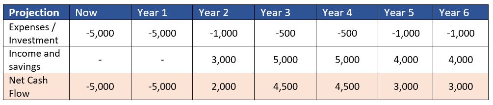
| Option 1 | Now | Year 1 | Year 2 | Year 3 | Year 4 | Year 5 | Year 6 |
| Expenses / Investment | -5,000 | -5,000 | -1,000 | -500 | -500 | -1,000 | -1,000 |
| Income and savings | – | – | 3,000 | 5,000 | 5,000 | 4,000 | 4,000 |
| Net Cash Flow | -5,000 | -5,000 | 2,000 | 4,500 | 4,500 | 3,000 | 3,000 |
| Option 2 | Now | Year 1 | Year 2 | Year 3 | Year 4 | Year 5 | Year 6 |
| Expenses / Investment | -15,000 | -1,000 | -1,000 | -1,000 | -500 | -500 | -1,000 |
| Income and savings | – | 2,500 | 5,000 | 5,000 | 5,000 | 5,000 | 5,000 |
| Net Cash Flow | -15,000 | 1,500 | 4,000 | 4,000 | 4,500 | 4,500 | 4,000 |
| Option 3 | Now | Year 1 | Year 2 | Year 3 | Year 4 | Year 5 | Year 6 |
| Expenses / Investment | -3,000 | -3,000 | -2,500 | -1,000 | -500 | -500 | -500 |
| Income and savings | – | – | 3,000 | 4,000 | 4,000 | 3,000 | 3,000 |
| Net Cash Flow | -3,000 | -3,000 | 500 | 3,000 | 3,500 | 2,500 | 2,500 |
The following table compares the net cash flows of all three options.
| Net Cash Flows | Now | Year 1 | Year 2 | Year 3 | Year 4 | Year 5 | Year 6 |
| Option 1 | -5,000 | -5,000 | 2,000 | 4,500 | 4,500 | 3,000 | 3,000 |
| Option 2 | -15,000 | 1,500 | 4,000 | 4,000 | 4,500 | 4,500 | 4,000 |
| Option 3 | -3,000 | -3,000 | 500 | 3,000 | 3,500 | 2,500 | 2,500 |
At first sight, Option 2 seems to be the most promising one, given its high benefits and early break-even point in year 1. Option 3, on the other hand, appears to be the least appealing alternative.
This perception is also reflected in the simple sums of cash flows for each option: 7,500 for Option 2, 7,000 for Option 1 and 6,000 for Option 3. However, the sum of non-discounted cash flows is not an appropriate type of value for comparing series of cash flows over time as it does not consider the points in time at which those cash flows occur. This is where the NPV method makes a difference.
Discounting Cash Flows and Calculating the NPV for Each Option
The next table contains discounted cash flows for each period and each option. They are calculated using the abovementioned formula, with the results summarized in the following tables.
| Option 1 | Now | Year 1 | Year 2 | Year 3 | Year 4 | Year 5 | Year 6 |
| Net Cash Flow | -5,000 | -5,000 | 2,000 | 4,500 | 4,500 | 3,000 | 3,000 |
| Formula for discounting cash flows | -5000 / (1 + 12%) ^ 0 | -5000 / (1 + 12%) ^ 1 | 2000 / (1 + 12%) ^ 2 | 4500 / (1 + 12%) ^ 3 | 4500 / (1 + 12%) ^ 4 | 3000 / (1 + 12%) ^ 5 | 3000 / (1 + 12%) ^ 6 |
| Discounted Net Cash Flow | -5,000 | -4,464 | 1,594 | 3,203 | 2,860 | 1,702 | 1,520 |
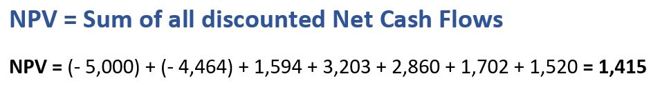
The Net Present Value (NPV) is the sum off all discounted cash flows:
NPV (Option 1) = (- 5,000) + (- 4,464) + 1,594 + 3,203 + 2,860 + 1,702 + 1,520 = 1,415
| Option 2 | Now | Year 1 | Year 2 | Year 3 | Year 4 | Year 5 | Year 6 |
| Net Cash Flow | -15,000 | 1,500 | 4,000 | 4,000 | 4,500 | 4,500 | 4,000 |
| Formula for discounting cash flows | -15000 / (1 + 12%) ^ 0 | 1500 / (1 + 12%) ^ 1 | 4000 / (1 + 12%) ^ 2 | 4000 / (1 + 12%) ^ 3 | 4500 / (1 + 12%) ^ 4 | 4500 / (1 + 12%) ^ 5 | 4000 / (1 + 12%) ^ 6 |
| Discounted Net Cash Flow | -15,000 | 1,339 | 3,189 | 2,847 | 2,860 | 2,553 | 2,027 |
NPV (Option 2) = (-185)
| Option 3 | Now | Year 1 | Year 2 | Year 3 | Year 4 | Year 5 | Year 6 |
| Net Cash Flow | -3,000 | -3,000 | 500 | 3,000 | 3,500 | 2,500 | 2,500 |
| Formula for discounting cash flows | -3000 / (1 + 12%) ^ 0 | -3000 / (1 + 12%) ^ 1 | 500 / (1 + 12%) ^ 2 | 3000 / (1 + 12%) ^ 3 | 3500 / (1 + 12%) ^ 4 | 2500 / (1 + 12%) ^ 5 | 2500 / (1 + 12%) ^ 6 |
| Discounted Net Cash Flow | -3,000 | -2,679 | 399 | 2,135 | 2,224 | 1,419 | 1,267 |
NPV (Option 3) = 1,765
Summary and Interpretation of Results
To compare the net present values and determine the best option (based on NPV), the alternatives are ranked by their NPV in descending order.
| Rank | Alternative | NPV |
| 1 | Option 3 | 1,765 |
| 2 | Option 1 | 1,415 |
| 3 | Option 2 | (-185) |
In this case, Option 3 is the most beneficial alternative, followed by Option 1. The benefits (inflows) of Option 2, on the other hand, do not even meet the expected rate of return which is indicated by a negative net present value.
These results are significantly different from the simple un-discounted sums calculated in the previous section. This proves, once again, how important the time factor and the interest rate are when it comes to assessing a series of cash flows.
Note that the NPV is only one part of a cost-benefit analysis. There may be qualitative criteria (for software, e.g. the company’s target IT architecture, security considerations, ease of use and maintenance, vendor rating etc.) as well as other calculation methods that could suggest a different ranking of those options.
Example 2) Calculating the NPV with a Perpetuity as Residual Value
The second example is an investment with a perpetuity as the residual value – a real estate investment, for instance.
The series starts with an initial investment of 1,000,000 that is incorporated as an outflow in year 0. The rental income is estimated at 60,000 in the first year with recurring cost (e.g. maintenance, management, taxes) of 10,000.
Both cash flow types are expected to increase by 2% each year. The detailed forecast covers 6 years with a residual value calculated based on future returns. The discount rate is 5% and may, for instance, represent the cost of funding and expected return.
The forecasted cash flows for the years 0 – 6 are as follows:
| Year | 0 | 1 | 2 | 3 | 4 | 5 | 6 |
| Investment and Cost (outflows) | -1,000,000 | -10,000 | -10,200 | -10,404 | -10,612 | -10,824 | -11,041 |
| Benefits and Earnings (inflows) | – | 60,000 | 61,200 | 62,424 | 63,672 | 64,946 | 66,245 |
| Net Cash Flow | -1,000,000 | 50,000 | 51,000 | 52,020 | 53,060 | 54,122 | 55,204 |
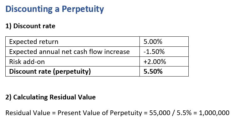
After year 6, the net cash flow is expected to be 55,000 with an expected annual growth of 1.5%. To account for the inherent insecurity of long-term estimates, a risk add-on of 2% is added to the expected return of 5%. The expected annual growth lowers the discount rate of the perpetuity (hence increases the present value) while the risk add-on increases the rate (and lowers the present value):
| Expected return | 5.00% |
| Expected annual net cash flow increase | -1.50% |
| Risk add-on | +2.00% |
| Discount rate (perpetuity) | 5.50% |
The perpetuity as the residual value is calculated by dividing the cash flow by the discount rate:
Residual Value = 55,000 / 5.5% = 1,000,000
This figure is the present value of the perpetuity at the end of year 6. It needs to be discounted – using the overall discount rate of 5% (alternatively, it could be discounted with 5.5% or any other discount rate) – along with all other cash flows.
Once all numbers are calculated, the table looks like this:
| Year | 0 | 1 | 2 | 3 | 4 | 5 | 6 | Residual Value |
| Investment & Cost (outflows) | -1,000,000 | -10,000 | -10,200 | -10,404 | -10,612 | -10,824 | -11,041 | |
| Benefits & Earnings (inflows) | – | 60,000 | 61,200 | 62,424 | 63,672 | 64,946 | 66,245 | |
| Net Cash Flow | -1,000,000 | 50,000 | 51,000 | 52,020 | 53,060 | 54,122 | 55,204 | |
| Residual Value | 1,000,000 | |||||||
| Formula for discounting cash flows | -1,000,000 / (1 + 5%) ^ 0 | 50,000 / (1 + 5%) ^ 1 | 51,000 / (1 + 5%) ^ 2 | 52,020 / (1 + 5%) ^ 3 | 53,060 / (1 + 5%) ^ 4 | 54,121 / (1 + 5%) ^ 5 | 55,204/ (1 + 5%) ^ 6 | 1,000,000 / (1 + 5%) ^ 6 |
| Discounted Net Cash Flow & RV | -1,000,000 | 47,619 | 46,259 | 44,937 | 43,653 | 42,406 | 41,194 | 746,215 |
The net present value of the investment is the sum of all discounted cash flows:
NPV = (-1,000,000) + 47,619 + 46,259 + 44,937 + 43,653 + 42,406 + 41,194 + 746,215 = 12,283
The positive NPV indicates a profitable investment.
Advantages and Disadvantages of the NPV
The net present value is a very common technique of cost-benefit analyses in finance, project management and various other economic areas. It takes the value of time and the expected return rate into account. One of the advantages for project managers and executives is that it produces only one figure per project and investment option that can easily be compared with other options. Lastly, it is fairly understandable which helps communicate the results of NPV-based cost benefit analyses.
However, the NPV comes with some disadvantages and weaknesses. It is broadly based on assumptions that can have a material, if not even game-changing, effect on the results. If the interest rate or the residual value are estimated, small changes to the parameters can heavily affect the present value. A methodological alignment of the calculation of different options and a high level of transparency on the assumptions can help reduce the risk of unintended or biased results. It also assumes that returns can be reinvested at the discount rate which might not always be the case in practice (source).
The net present value aggregates a number of estimates into one catchy figure. While this increases understandability and keeps things comparable and manageable, the information on the duration of the repayment of an initial investment is lost. Irrespective of economic figures, some decision-makers might prefer an option with high returns in early periods over an option with a higher NPV but returns coming in in later periods. This distinction is not possible when comparing project options solely based on the NPV.
Conclusion
The Net Present Value is a popular method of cost-benefit analyses as it is comparatively easy to understand and provides an accurate basis for comparing different project or investment alternatives. However, it requires a set of assumptions and comes with a number of weaknesses – one of which is the usually rough calculation yet high relevance of residual values for long-term investments.
Therefore, you should always maintain a critical view on the results and assumptions of NPV calculations. For investment decisions, it is not recommended to rely on only one single indicator. You should in fact use other quantitative and qualitative methods to assess alternative options as well.