
Estimating time, efforts and cost is one of the most critical parts of project management. This is because of the fundamental importance of these estimates for the entire project planning and, in particular, the scope, schedule and cost baseline. One of the estimation techniques suggested in the PMI Project Management Body of Knowledge (PMBOK 6th ed., ch. 6.4, 7.2) is the three-point estimate used with the triangular, Beta or PERT distribution. We will introduce these methods in this article.
What Is the Three-Point Estimation Technique?
The three-point estimate is a simple yet useful approach to estimating the time or cost of work items. According to the PMI methodology, it is used in the process groups “Estimate Activity Duration” and “Estimate Costs”. The technique involves three different estimates that are usually obtained from subject matter experts:
- Optimistic estimate,
- Pessimistic estimate,
- Most likely estimate.
The optimistic estimate is the expected amount of work or time needed to perform an activity assuming no impediments occur and everything is going smooth. It represents the so-called best-case scenario. The pessimistic point is based on the assumption that the opposite was true – it represents the worst-case scenario. Although both estimates are referring to the extreme points of the range of expected outcomes, the estimates are supposed to be somewhat realistic.
The third point reflects the most likely case, it is the estimation of work or time that is deemed to be the most realistic. One could be tempted to simply use the mean between the optimistic and pessimistic points without giving it a second thought. However, this may not be appropriate for many cases. In practice, it is normally worthwhile to determine this most likely estimate properly, analogous the other estimation points.
The result of three-point estimating is a so-called triangular distribution of time values or cost amounts, comprising of the three estimates (see illustration below).
What Is PERT?
PERT stands for Program Evaluation and Review Technique and was developed as an advanced project schedule planning and management system by the US navy in the 1950s (source: Heldman, PMP Study guide, ch. 4).
Another, not too serious, story of its origination was once published by an anonymous author in PMI’s journal (see: Anonymous (1975). PERT—the hoax of the century. Project Management Quarterly, 6(3), 22–23).
In PMI-style projects, PERT is primarily used as a supplemental technique to the Critical Path Method for scheduling activities. However, it can also be applied to stand-alone estimates of work items and activities.
The so-called PERT distribution leverages on the values determined with the three-point estimation technique. It can basically be used for all planning levels, ranging from activities to entire projects. However, finding the right granularity for meaningful estimating may require some critical and conceptual thinking.
The PERT method implies overweighting the ‘most likely’ estimate. It transforms the three-point estimate into a bell-shaped curve and allows to determine probabilities of ranges of expected values.
What Are the Differences between Triangular and PERT Distribution of Three-Point Estimates?
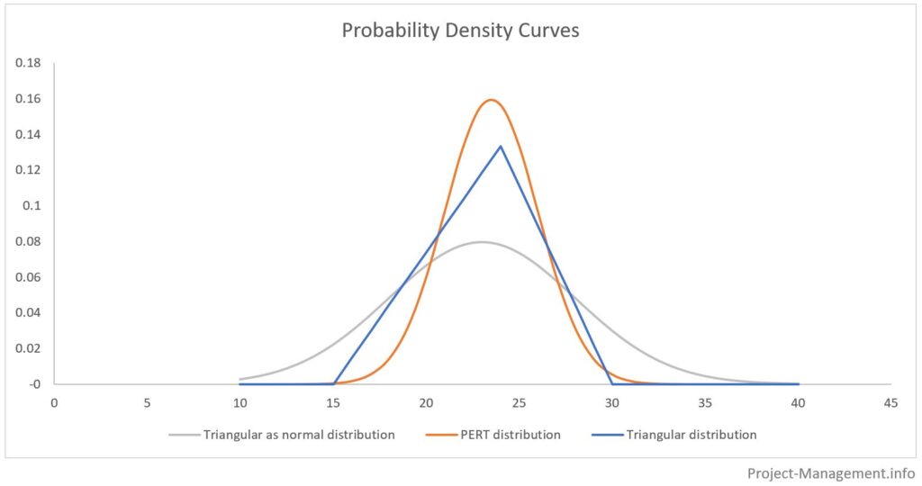
While the triangular distribution only considers the three estimated points, the PERT method allows to convert the three-point estimate into a bell-shaped, nearly normally distributed curve. Thus, it can be used for the calculation of probabilities of ranges of expected durations.
The following diagram illustrates the differences between the PERT distribution, the triangular distribution and a presentation of the three-point estimate as if it were a normal distribution.
The areas under the probability distribution curves represent the cumulative probabilities of the respective ranges of estimates. Typically, these ranges are determined with the expected value +/- standard deviation multiplied by 1, 2 and 3. This is illustrated in the following figure:
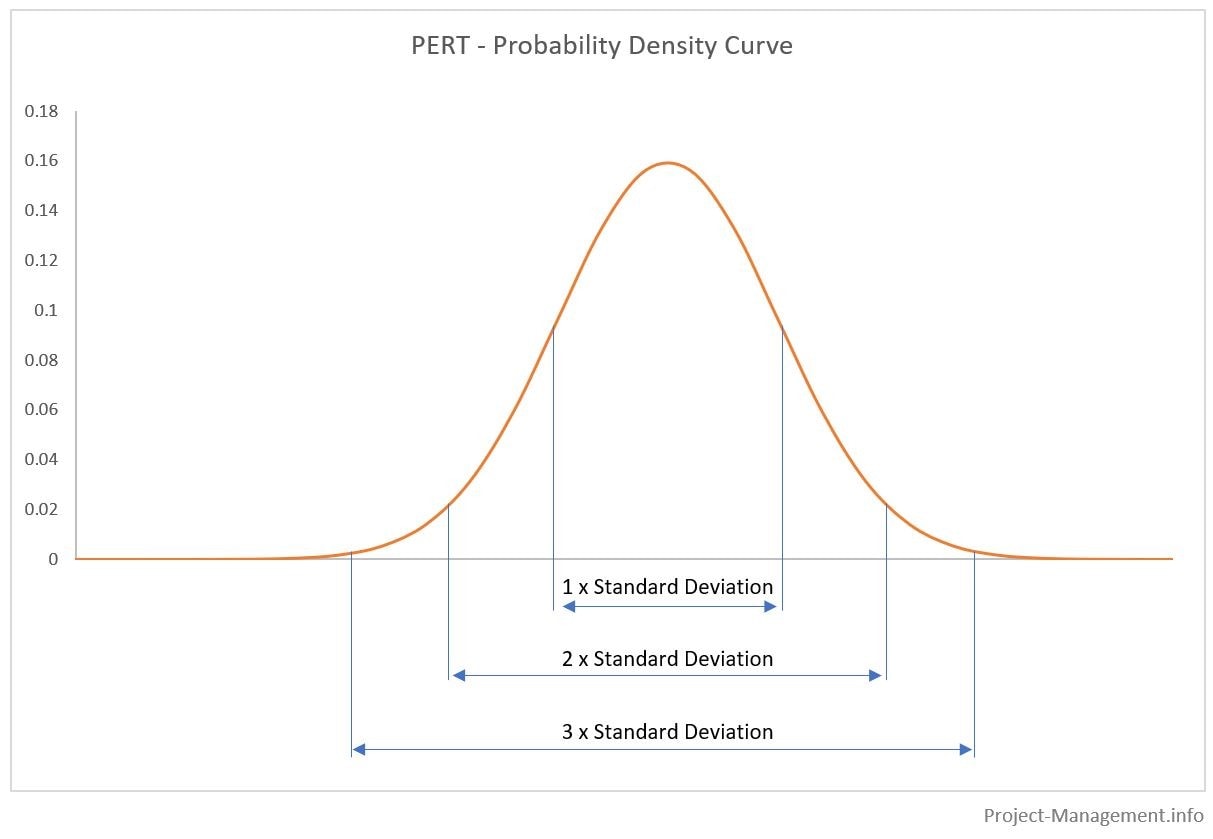
The resulting probabilities (approx.) are
- 68.3% for 1 standard deviation,
- 95.5% for 2 standard deviations,
- 99.7% for 3 standard deviations.
The knowledge required for the PMP exam is limited to calculating the expected estimates and being familiar with the different probabilities (source). Therefore, we will not cover the statistical details and background in this article – you can find those details on Riskamp.
Use this calculator to determine the three-point estimates and PERT.
How Is Three-Point Estimate Calculated?
The Triangular Distribution
The simple yet commonly used calculation involves the average or mean of the 3 estimated values. The formula of this triangular distribution is:
E = (O + M + P) / 3
where:
E = Expected amount of time or cost,
O = Optimistic estimate,
M = Most likely estimate,
P = Pessimistic estimate.
The PMBOK uses t(E), t(O), t(M) and t(P) as variables for time estimates and c(E), c(O), c(M) and c(P).
The weight of each estimate in this equation is identical. Thus, the ‘most likely’ case does not affect the final estimate more than the 2 less likely estimates. This is different from the beta distribution method.
The PERT Beta Distribution
The PERT beta distribution takes into account that the ‘most likely’ case is more likely to occur which is reflected in a multiplier for that estimate. The PMI methodology suggests this calculation as an alternative to the triangular distribution for cost estimates (however, we are of the view that it can also be used for time estimates).
In this method, the most likely estimate receives a multiplier of 4 while the overall divisor is increased to 6. The formula is as follows:
E = (O + 4*M + P) / 6
where:
E = Expected amount of time or cost,
O = Optimistic estimate,
M = Most likely estimate,
P = Pessimistic estimate.
The Standard Deviation of the PERT distribution is calculated using the formula:
Standard Deviation = (P – O) / 6
For estimating an entire path (analogous critical path method), a similar concept is applied yet using a combined standard deviation of all activities.
Example of a Three-Point Estimate and PERT
A team of subject matter experts is estimating the time it takes to complete an activity. In this example, the duration of an activity is estimated using the three-point estimating technique. They come up with the following numbers:
| Optimistic estimate | 15 days |
| Pessimistic estimate | 24 days |
| Most likely estimate | 30 days |
The values range from 15 days (optimistic) to 30 days (pessimistic). A duration of 24 days is deemed to be the most likely amount of time needed for the completion of the work.
Calculating the Expected Duration with a Triangular Distribution
The expected duration using a triangular distribution is calculated as follows:
Final Estimate = (15 + 30 + 24) / 3.
The resulting final estimate under this method is 23, which is basically the unweighted average of the 3 estimates.
Calculating the Expected Duration Using PERT Beta Distribution
The expected duration can also be calculated with the PERT method:
Final Estimate (expected value) = (15 + 4×24 + 30) / 6.
The resulting expected value is 23.5 days which is greater than the final estimate determined under the triangular method. This is due to the higher weight (i.e. the multiplier of 4) that is assigned to the ‘most likely’ estimate.
The standard deviation of this estimation is:
Standard Deviation = (30 – 15) / 6 = 2.5
Determining the Probabilities of the Expected Duration
Having calculated the expected duration and the standard deviation enables the project manager to determine the probabilities (approx.):
| Range | Probability | Lower Boundary | Upper Boundary |
| 1 x standard deviation | 68.3% | 21 [= 23.5 – 2.5] | 26 [= 23.5 + 2.5] |
| 2 x standard deviation | 95.5% | 18.5 [= 23.5 – 2 x 2.5] | 28.5 [= 23.5 + 2 x 2.5] |
| 3 x standard deviation | 99.7% | 16 [= 23.5 – 3 x 2.5] | 31 [= 23.5 + 3 x 2.5] |
With 68.3% probability, the duration of the activity will be between 21 and 26 days. For a range of 18.5 to 28.5 days, the probability is 95.5%. Using 3 standard deviations covers almost the entirety of all data points and determines a 99.7%-probability that the duration will eventually be between 16 and 31 days.
Summary
The final estimate under the triangular method was 23, compared to 23.5 using the PERT method. This is because the latter assigns a higher weighing to the ‘most likely’ case which, in our case, is not exactly the mean (or unweighted average) of the optimistic and pessimistic estimate.
Using the PERT method allows taking probabilities of value ranges into account. This is useful if the quality of estimates varies, e.g. if the difference between optimistic and pessimistic estimates is significantly deviating among different activities. In this case, using ranges and their probabilities will reflect the scattering and level of confidence of the underlying estimates.
Conclusion
The estimation of activities with respect to their time and cost requirements is crucial for the planning and scheduling of projects and activities. In many projects, more accurate estimates, such as parametric estimates, based on statistical correlations of comparable projects in the past, for instance, are not available. The three-point estimation technique offers a good approach to processing and balancing top-down or subject matter expert estimates in such situations.
The PERT distribution is probably the most accurate method to aggregate these worst, best and most likely cases into a single figure (expected value) or a range of values. Thanks to the use of the standard deviation, it takes both the inherent uncertainties and the potential scattering of estimates into account.
This might be the reason why PERT is still a common method in project estimation and scheduling although it has been around for some decades and could already have been used by our grandparents (if they had been project managers).